Regression: Allgemeine Gleichung 2. Ordnung
Quellen
Wikipedia : Carl Friedrich GaußWikipedia : Gaußsches Eliminationsverfahren
Wikipedia : Cramersche Regel
OpenHardSoftWare.de : Cramersche Regel
Download als PDF-Dokument : 2206181041_GeneralEquation2ndOrder.pdf
Übersicht
Allgemeine Gleichung 2. Grades in impliziter Form:$\boxed{F(x, y) = a x^2 + b y^2 + c x y + d x + e y - 1}$ (1)
mit $a, b, c, d, e \in \mathbb{R}$ und $x, y \in \mathbb{R}$
$\boxed{F_{theory}(x, y) = a x^2 + b y^2 + c x y + d x + e y - 1}$ (1.1)
$\boxed{F_{measure}(x_i, y_i) = a x_i^2 + b y_i^2 + c x_i y_i + d x_i + e y_i - 1}$ (1.2)
Dabei gilt die Nicht-Identität für alle gegebenen Punkte: $\forall P_i(x_i, y_i) \neq \forall P_j(x_j, y_j)$
mit $N$ : Anzahl der Punkte $P_i$ und $i, j \in [5, .. , N]$
Herleitung
Allgemeine Gleichung 2. Grades:$F^\star(x, y) = 0 = a^\star x^2 + b^\star y^2 + c^\star x y + d^\star x + e^\star y + f^\star$
Identisch zu (Division durch $-f$):
$\boxed{F(x, y) := a x^2 + b y^2 + c x y + d x + e y - 1}$ (1)*
ohne Einschränkung der Allgemeinheit. Damit gilt es, die (linearen) Koeffizienten $a, b, c, d, e$
zu bei einer gegebenen Punktemenge $P_i = (x_i, y_i)$ zu berechnen.
Die "Methode der kleinsten Fehlerquadrate" nach Carl Friedrich Gauss liefert folgenden Ansatz:
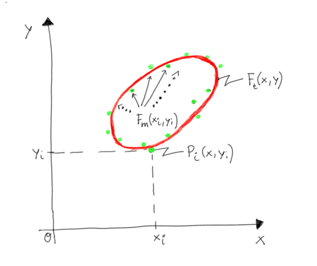
$\boxed{S = \sum\limits_{i=1}^{N}{\bigg[F_m(x, y) - F_t(x, y)\bigg]^2}}$ (2)
mit: $F_{theory}(x, y) = F_t(x, y) = a x^2 + b y^2 + c x y + d x + e y - 1 = 0$ (1.1)*
und: $F_{measure}(x, y) = F_m(x_i, y_i) = a x_i^2 + b y_i^2 + c x_i y_i + d x_i + e y_i - 1$ (1.2)*
ergibt sich:
$S = \sum\limits_{i=1}^{N}{\bigg[ F_m(x_i, y_i) - F_t(x, y) \bigg]^2}$
$S = \sum\limits_{i=1}^{N}{\bigg[ F_m(x_i, y_i) - 0 \bigg]^2}$
$S = \sum\limits_{i=1}^{N}{\bigg[ F_m(x_i, y_i) \bigg]^2}$
$\boxed{S = \sum\limits_{i=1}^{N}{\bigg[ a x_i^2 + b y_i^2 + c x_i y_i + d x_i + e y_i - 1 \bigg]^2}}$ (3)
Notwendige Bedingungen, damit die Koeffizienten $a, b, .. ,e$ optimal mit kleinstem Fehler
durch die Punkte $P_i(xi, y_i)$ gefittet werden:
$\dfrac{\partial S}{\partial a} = 0 = 2 \sum\limits_i \big[ a x_i^2 + b y_i^2 + c x_i y_i + d x_i + e y_i - 1 \big]\big[ x_i^2 \big]$
$\dfrac{\partial S}{\partial b} = 0 = 2 \sum\limits_i \big[ a x_i^2 + b y_i^2 + c x_i y_i + d x_i + e y_i - 1 \big]\big[ y_i^2 \big]$
$\dfrac{\partial S}{\partial c} = 0 = 2 \sum\limits_i \big[ a x_i^2 + b y_i^2 + c x_i y_i + d x_i + e y_i - 1 \big]\big[ x_i y_i \big]$
$\dfrac{\partial S}{\partial d} = 0 = 2 \sum\limits_i \big[ a x_i^2 + b y_i^2 + c x_i y_i + d x_i + e y_i - 1 \big]\big[ x_i \big]$
$\dfrac{\partial S}{\partial e} = 0 = 2 \sum\limits_i \big[ a x_i^2 + b y_i^2 + c x_i y_i + d x_i + e y_i - 1 \big]\big[ y_i \big]$
$\dfrac{\partial S}{\partial a} = 0 = \sum\limits_i \big[ a x_i^4 + b x_i^2 y_i^2 + c x_i^3 y_i + d x_i^3 + e x_i^2 y_i - x_i^2 \big]$
$\dfrac{\partial S}{\partial b} = 0 = \sum\limits_i \big[ a x_i^2 y_i^2 + b y_i^4 + c x_i y_i^3 + d x_i y_i^2 + e y_i^3 - y_i^2 \big]$
$\dfrac{\partial S}{\partial c} = 0 = \sum\limits_i \big[ a x_i^3 y_i + b x_i y_i^3 + c x_i^2 y_i^2 + d x_i^2 y_i + e x_i y_i^2 - x_i y_i \big]$
$\dfrac{\partial S}{\partial d} = 0 = \sum\limits_i \big[ a x_i^3 + b x_i y_i^2 + c x_i^2 y_i + d x_i^2 + e x_i y_i - x_i \big]$
$\dfrac{\partial S}{\partial e} = 0 = \sum\limits_i \big[ a x_i^2 y_i + b y_i^3 + c x_i y_i^2 + d x_i y_i + e y_i^2 - y_i \big]$
$a\sum\limits_i x_i^4 + b \sum\limits_i x_i^2 y_i^2 + c \sum\limits_i x_i^3 y_i + d \sum\limits_i x_i^3 + e \sum\limits_i x_i^2 y_i = \sum\limits_i x_i^2$
$a \sum\limits_i x_i^2 y_i^2 + b \sum\limits_i y_i^4 + c \sum\limits_i x_i y_i^3 + d \sum\limits_i x_i y_i^2 + e \sum\limits_i y_i^3 = \sum\limits_i y_i^2$
$a \sum\limits_i x_i^3 y_i + b \sum\limits_i x_i y_i^3 + c \sum\limits_i x_i^2 y_i^2 + d \sum\limits_i x_i^2 y_i + e \sum\limits_i x_i y_i^2 = \sum\limits_i x_i y_i$
$a \sum\limits_i x_i^3 + b \sum\limits_i x_i y_i^2 + c \sum\limits_i x_i^2 y_i + d \sum\limits_i x_i^2 + e \sum\limits_i x_i y_i = \sum\limits_i x_i$
$a \sum\limits_i x_i^2 y_i + b \sum\limits_i y_i^3 + c \sum\limits_i x_i y_i^2 + d \sum\limits_i x_i y_i + e \sum\limits_i y_i^2 = \sum\limits_i y_i$
Daher folgt ein lineares Gleichungssystem der Unbekannten $a, b, c, d, e$ :
$ \begin{pmatrix} a & b & c & d & e & iT\\ \sum\limits_i x_i^4 & \sum\limits_i x_i^2 y_i^2 & \sum\limits_i x_i^3 y_i & \sum\limits_i x_i^3 & \sum\limits_i x_i^2 y_i & \sum\limits_i x_i^2 \\ \sum\limits_i x_i^2 y_i^2 & \sum\limits_i y_i^4 & \sum\limits_i x_i y_i^3 & \sum\limits_i x_i y_i^2 & \sum\limits_i y_i^3 & \sum\limits_i y_i^2 \\ \sum\limits_i x_i^3 y_i & \sum\limits_i x_i y_i^3 & \sum\limits_i x_i^2 y_i^2 & \sum\limits_i x_i^2 y_i & \sum\limits_i x_i y_i^2 & \sum\limits_i x_i y_i \\ \sum\limits_i x_i^3 & \sum\limits_i x_i y_i^2 & \sum\limits_i x_i^2 y_i & \sum\limits_i x_i^2 & \sum\limits_i x_i y_i & \sum\limits_i x_i \\ \sum\limits_i x_i^2 y_i & \sum\limits_i y_i^3 & \sum\limits_i x_i y_i^2 & \sum\limits_i x_i y_i & \sum\limits_i y_i^2 & \sum\limits_i y_i \end{pmatrix} $
Die Lösungen für $a, b, c, d, e$ ergeben sich prinzipiell aus der Cramerschen Regel:
$\boxed{a = \dfrac{D_a}{D}}$ $\boxed{b = \dfrac{D_b}{D}}$ $\boxed{c = \dfrac{D_c}{D}}$ $\boxed{d = \dfrac{D_d}{D}}$ $\boxed{e = \dfrac{D_e}{D}}$
Da die Anzahl der Unbekannten $a, b, c, d, e$ die Zahl 4 überschreitet, eignet sich das
Gaußsche Eliminationsverfahren zur effizienten Bestimmung der Unbekannten.
WebSites Module Mathematik